ARTIST Tutorial: Surface Reconstruction

Note

You can find the corresponding Python script for this tutorial here: https://github.com/ARTIST-Association/ARTIST/blob/main/tutorials/03_nurbs_surface_reconstruction_tutorial.py

This tutorial demonstrates how a heliostat surface can be reconstructed using Non-Uniform Rational B-Splines (NURBS) in ARTIST. It introduces the key steps involved in the reconstruction workflow, including:

• loading the data required for surface reconstruction,

• defining the loss functions and regularizers used during optimization,

• configuring the optimizer and learning rate scheduler, and

• performing the surface reconstruction.

Before starting this tutorial, make sure you are familiar with how to load a scenario, run ARTIST in a distributed environment, and understand the structure of a scenario.

If you are not using your own scenario, we recommend using the test_scenario_paint_multiple_heliostat_groups_ideal.h5 scenario provided in the scenarios/ folder.

Loading Data

As a first step, you must load the calibration properties and flux images data required for reconstructing the surfaces. This information is specified in the heliostat_data_mapping list. Each entry in this list is a tuple containing the heliostat name and the paths to its calibration data, which include both a calibration properties .json file and a .png flux image.

If you are not using your own data, you can use the sample data provided in the data/ directory. For example, the data for heliostats AA31, AA39, and AC43 will work with the test_scenario_paint_multiple_heliostat_groups_ideal.h5 scenario:

# Specify the heliostats to be calibrated and the paths to your calibration-properties.json files.
# Please use the following style: list[tuple[str, list[pathlib.Path], list[pathlib.Path]]]
heliostat_data_mapping = [
    (
        "heliostat_name_1",
        [
            pathlib.Path(
                "please/insert/the/path/to/the/paint/data/here/calibration-properties.json"
            ),
            # ....
        ],
        [
            pathlib.Path("please/insert/the/path/to/the/paint/data/here/flux.png"),
            # ....
        ],
    ),
    (
        "heliostat_name_2",
        [
            pathlib.Path(
                "please/insert/the/path/to/the/paint/data/here/calibration-properties.json"
            ),
            # ....
        ],
        [
            pathlib.Path("please/insert/the/path/to/the/paint/data/here/flux.png"),
            # ....
        ],
    ),
    # ...
]

This mapping is stored in a data dictionary together with the data parser. Later on, the dictionary will be used during the optimization process:

# Create dict for the data parser and the heliostat_data_mapping.
data: dict[
    str,
    CalibrationDataParser | list[tuple[str, list[pathlib.Path], list[pathlib.Path]]],
] = {
    constants.data_parser: PaintCalibrationDataParser(sample_limit=2),
    constants.heliostat_data_mapping: heliostat_data_mapping,
}

Next, you can load the scenario and set up the distributed environment as in the previous tutorials.

Setting up the Optimization

Surface reconstruction in ARTIST is framed as an optimization problem. The goal is to reconstruct a heliostat surface whose simulated flux distribution matches the measured calibration data. To achieve this, we define

• a loss function to measure the difference between the simulated flux distribution of the reconstructed surface and the measured calibration data, as well as

• regularizers that enforce physically meaningful surfaces, and

• constraints that stabilize the optimization process.

Loss Functions

In this tutorial we use the KLDivergenceLoss as the loss function. This loss measures the difference between two probability distributions. In our case, the measured flux density image used as the target is interpreted as a discrete probability distribution and serves as the reference distribution. Alternatively, you can use the PixelLoss which compares the simulated and measured flux images pixel-wise.

# Set loss function.
loss_definition = KLDivergenceLoss()

Optimizer, Scheduler, Regularizer, and Constraints Configuration

The surface reconstruction internally uses the torch.optim.Adam optimizer. Depending on the dataset and reconstruction problem, different optimizer parameters and learning rate schedulers may lead to better results. Below, we configure the optimizer parameters and define the learning rate scheduler. In this example, we use an exponential scheduler. In practice, cyclic or reduce-on-plateau schedulers have also achieved good results.

# Configure the optimizer.
optimizer_dict = {
    constants.initial_learning_rate: 1e-4,
    constants.tolerance: 1e-5,
    constants.max_epoch: 30,
    constants.batch_size: 30,
    constants.log_step: 1,
    constants.early_stopping_delta: 1e-4,
    constants.early_stopping_patience: 100,
    constants.early_stopping_window: 100,
}
# Configure the learning rate scheduler.
scheduler_dict = {
    constants.scheduler_type: constants.exponential,
    constants.gamma: 0.99,
    constants.lr_min: 1e-6,
    constants.lr_max: 1e-2,
    constants.step_size_up: 100,
    constants.reduce_factor: 0.5,
    constants.patience: 10,
    constants.threshold: 1e-4,
    constants.cooldown: 5,
}

Regularizers are used to prevent overfitting and ensure that the reconstructed surface is smooth and remains physically plausible, i.e., similar to an ideal surface. We use two regularizers in the surface reconstruction:

IdealSurfaceRegularizer

Pushes the reconstructed surface towards the shape of an ideal, perfectly flat or canted surface. Since the overall surface shape is typically known from the heliostat design, the reconstruction mainly focuses on small local deformations. This regularizer therefore discourages unrealistic large deviations from an ideal surface.

SmoothnessRegularizer

Promotes smooth surfaces by penalizing large gradients between neighboring control points. The assumption is that real heliostat surfaces deform smoothly, making abrupt surface variations physically unlikely.

These regularizers are initialized automatically within the SurfaceReconstructor. Their influence can be controlled through the weights specified in the constraints dict. Setting a weight to zero disables the corresponding regularizer.

# Configure the regularizers and constraints.
constraint_dict = {
    constants.weight_smoothness: 0.005,
    constants.weight_ideal_surface: 0.005,
    constants.rho_flux_integral: 1.0,
    constants.energy_tolerance: 0.01,
}

In addition to the regularizers, ARTIST applies an energy conservation constraint to further stabilize the reconstruction. This constraint ensures that the total flux integral of the simulated flux images does not change significantly during optimization.

The parameter rho_flux_integral is a coefficient of an Augmented Lagrangian formulation used to enforce this constraint. To understand the Augmented Lagrangian formulation, consider the parameter lambda_flux_integral which is set automatically inside the MotorPositionsOptimizer. This is the Lagrange multiplier associated with the flux integral constraint. It linearly penalizes deviations from the reference flux integral and is updated iteratively during the optimization based on the current constraint violation. If the simulated energy deviates more strongly from the reference energy, lambda_energy increases, thereby strengthening the enforcement of the constraint in the next iteration. For the constraint_dict we need to define:

rho_flux_integral

The quadratic penalty weight controlling the strength of the squared constraint term.

energy_tolerance

Specifies how much the flux integral may deviate relative to the initial surface.

Together, these parameters ensure that the reconstructed surface produces a flux distribution with a physically consistent total energy.

We can now combine all optimization parameters in the optimization_configuration dictionary:

optimization_configuration = {
    constants.optimization: optimizer_dict,
    constants.scheduler: scheduler_dict,
    constants.constraints: constraint_dict,
}

Note

The parameters shown above have performed well for our data and experiments. However, optimal settings may vary depending on the calibration data and reconstruction scenario.

Performing Surface Reconstruction

Now we are almost ready to perform the surface reconstruction. Since ARTIST internally uses ray tracing to generate the flux images required for the loss calculation, we need to define several ray-tracing parameters. In particular, we specify the number_of_rays, the number_of_surface_points, and the bitmap resolution. These parameters control the resolution of the simulated flux images. Increasing them generally improves reconstruction accuracy but also increases computation time.

scenario.set_number_of_rays(number_of_rays=120)
number_of_surface_points = torch.tensor([100, 100], device=device)
resolution = torch.tensor([256, 256], device=device)

With these parameters defined, we can instantiate a SurfaceReconstructor and start the optimization:

# Create the surface reconstructor.
surface_reconstructor = SurfaceReconstructor(
    ddp_setup=ddp_setup,
    scenario=scenario,
    data=data,
    optimization_configuration=optimization_configuration,
    number_of_surface_points=number_of_surface_points,
    bitmap_resolution=resolution,
    device=device,
)

# Reconstruct surfaces.
final_loss_per_heliostat, _ = surface_reconstructor.reconstruct_surfaces(
    loss_definition=loss_definition, device=device
)

During this process, the NURBS parameters defining the heliostat surface are optimized and stored directly in the scenario. The reconstruct_surfaces() method returns the loss per heliostat, which can be used to evaluate the reconstruction quality.

What Does Surface Reconstruction Do?

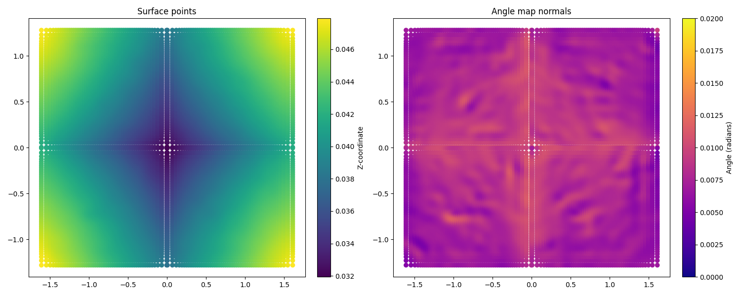
To better understand the effect of surface reconstruction, consider two heliostats that are initially loaded with ideal surfaces (here referred to as Heliostat 1 and Heliostat 2):

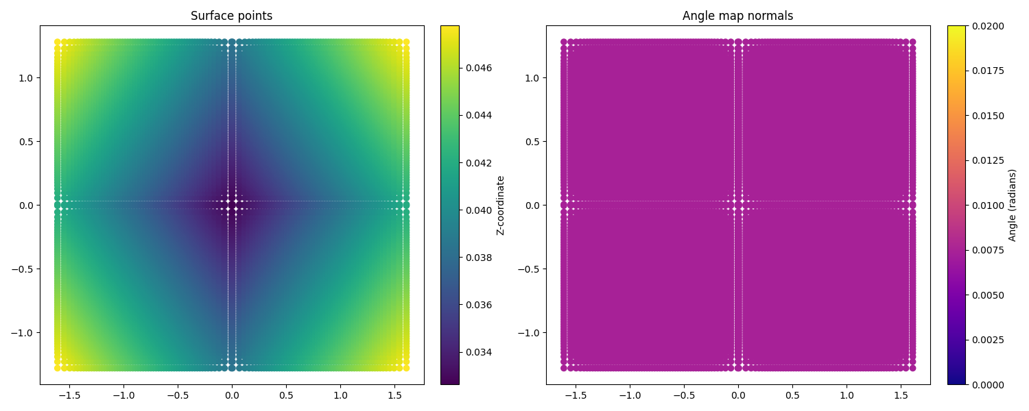
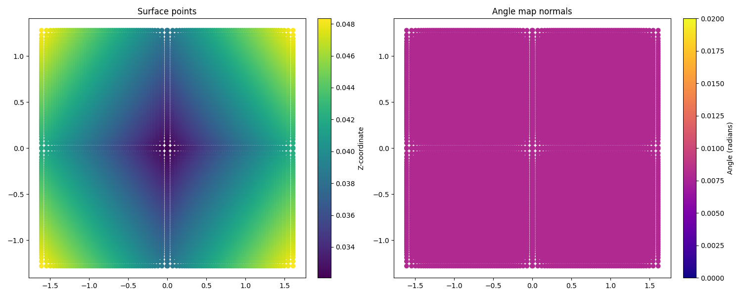
The left side shows the coordinates of the surface points, with the z coordinate highlighted by the color scale. As expected, the heliostats appear almost perfectly square, and the variation in z indicates the canting of the facets.

The right side shows the surface normals. The color scale indicates the angle between each normal and a reference direction. Because the surfaces are ideal, all normals have identical angles and no deformations are visible.

However, this situation is not realistic. When we compare the simulated flux images produced by these ideal surfaces with the measured target images, we see that they do not match at all:

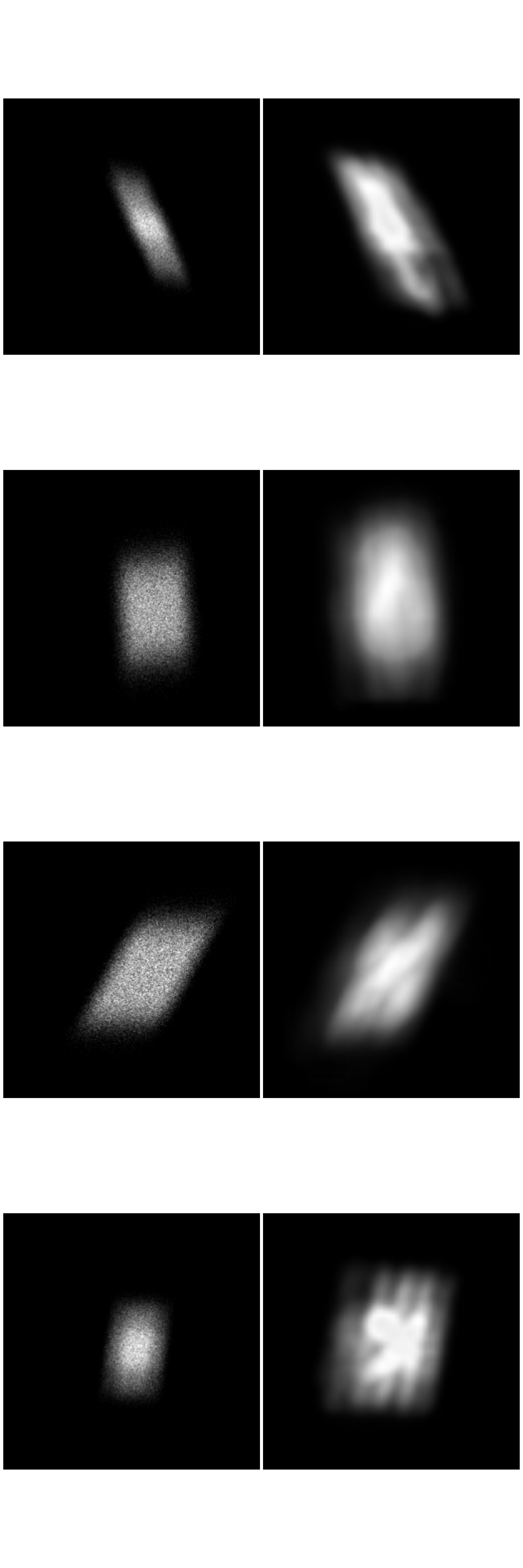
Although the overall shape of the flux distribution is captured, the internal structure of the flux pattern is missing. This indicates that the real heliostat surfaces deviate from the ideal model. After performing surface reconstruction, the surfaces of both heliostats adapt to better match the measured data:

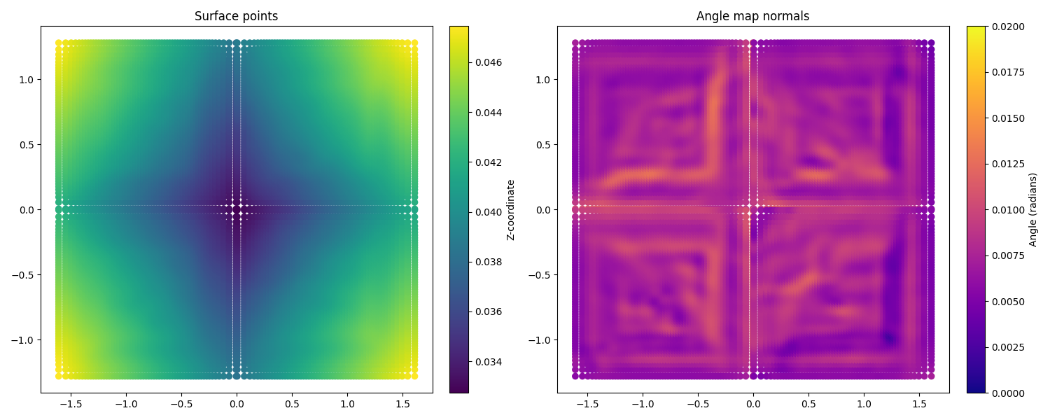
While the surface points have only changed marginally, the surface normals now exhibit clear deviations. These changes correspond to learned surface deformations that better represent the real heliostat geometry.

The resulting flux images reflect these improvements:

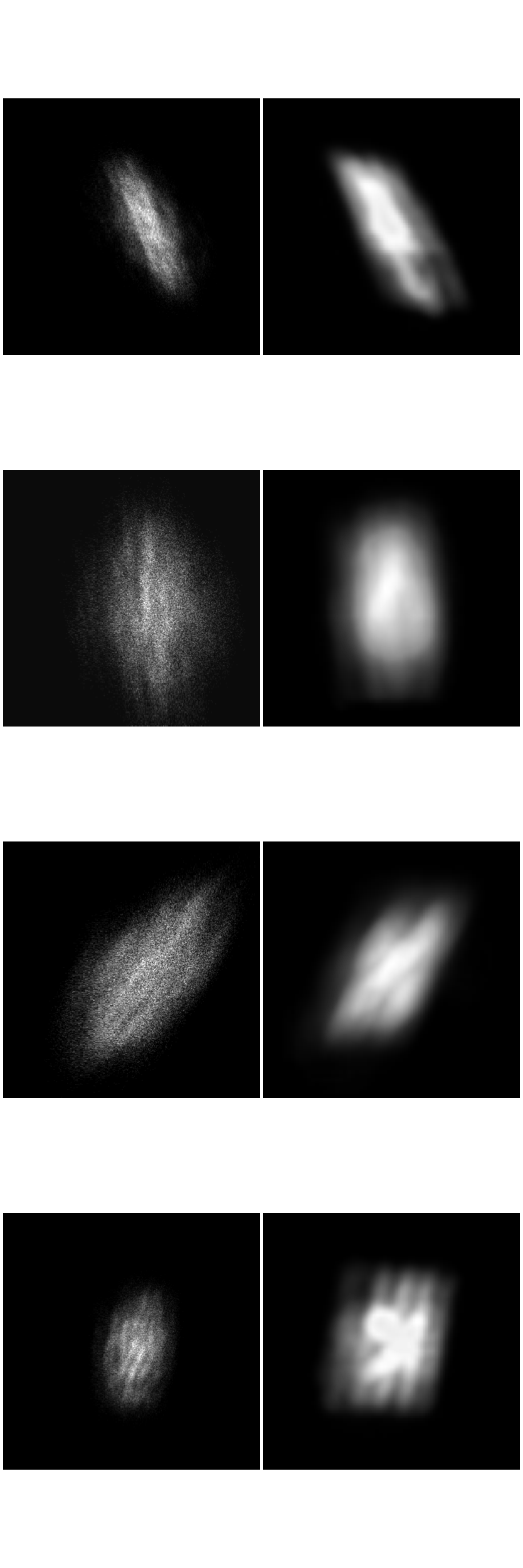
The reconstructed surfaces capture significantly more detail in the flux distribution. In practice, the reconstruction quality can be further improved by adjusting hyperparameters, using a more realistic sun model, or increasing the number of rays used in the simulation. Heliostat surface reconstruction is a crucial step when creating a digital twin of a solar tower power plant, as is allows the simulated optical behavior to match the real system more accurately.

That is all there is to surface reconstruction in ARTIST – hopefully this helped you understand how the process works and the importance of this step.

Note

The images generated in this tutorial are for illustrative purposes, often with reduced resolution and without hyperparameter optimization. Therefore, they should not be taken as a quality measure for ARTIST. Please see our publications for further information.