`ARTIST` Tutorial: Motor Position Optimization

Note

You can find the corresponding Python script for this tutorial here: https://github.com/ARTIST-Association/ARTIST/blob/main/tutorials/05_motor_positions_optimizer_tutorial.py

This tutorial demonstrates how to optimize heliostat motor positions in ARTIST, which is a crucial step for precise heliostat alignment and maximizing power plant efficiency.

The tutorial will walk you through the key concepts needed to perform this optimization, including:

Defining the ground truth and the loss function,
configuring the optimization parameters, and
performing the motor positions optimization.

Before starting, make sure you know how to load a scenario, run ARTIST in a distributed environment, and understand the structure of a scenario. If you are not using your own scenario, we recommend using either

test_scenario_paint_multiple_heliostat_groups_deflectometry.h5 or
test_scenario_paint_multiple_heliostat_groups_ideal.h5

provided in the scenarios/ folder.

You should also have your scenario loaded and the distributed environment set up, as shown in previous tutorials.

Motor Position Optimization

Motor position optimization adjusts the motor positions of all heliostats in the field to achieve a desired flux distribution on the solar tower. In this tutorial, we target a trapezoid distribution on the receiver, i.e., all regions should get approximately the same amount of sunlight. The resulting optimal flux density distribution maximizes the plant’s energy yield and prevents local overheating.

Below, we define the targeted trapezoid distribution as the ground truth:

e_trapezoid = bitmap.trapezoid_distribution(
    total_width=256, slope_width=30, plateau_width=110, device=device
)
u_trapezoid = bitmap.trapezoid_distribution(
    total_width=256, slope_width=30, plateau_width=110, device=device
)
ground_truth = u_trapezoid.unsqueeze(
    index_mapping.unbatched_bitmap_u
) * e_trapezoid.unsqueeze(index_mapping.unbatched_bitmap_e)

Flux Scaling

As we typically want to maximize the energy on the receiver while optimally distributing the single heliostat fluxes, the flux integral is an essential quantity in motor position optimization. To simulate the energy on the receiver, each ray needs to be assigned a meaningful magnitude. This is done by providing the dni parameter in the MotorPositionsOptimizer. The direct normal irradiance (DNI) is the insolation at a given location on Earth with a surface element perpendicular to the sun’s rays, excluding diffuse insolation. It is provided in W/m^2 and automatically converted to ray magnitudes.

For the optimization, the targeted ground_truth distribution is scaled with the scalar target_flux_integral value:

# Set target flux integral.
canting_norm = (
    torch.norm(scenario.heliostat_field.heliostat_groups[0].canting[0], dim=1)[0]
)[:2]
dimensions = (canting_norm * 4) + 0.02
heliostat_surface_area = dimensions[0] * dimensions[1]
total_heliostat_area = (
    heliostat_surface_area
    * scenario.heliostat_field.number_of_heliostats_per_group.sum()
)
target_flux_integral = (
    dni * total_heliostat_area * 0.75
)  # Account for mirror and angle based losses.

Loss Function

We again use the KLDivergenceLoss as the loss function:

loss_definition = KLDivergenceLoss()

The KLDivergenceLoss measures the difference between the predicted flux distribution generated by all heliostats in the scenario and the reference trapezoid distribution.

Optimization Configuration

Before we can perform the optimization, we need to define the optimization configuration. Internally, ARTIST uses the torch.optim.Adam optimizer. We use the following scheduler and optimization settings:

# Set optimizer parameters.
optimizer_dict = {
    constants.initial_learning_rate: 3e-4,
    constants.tolerance: 0.0005,
    constants.max_epoch: 100,
    constants.batch_size: 50,
    constants.log_step: 3,
    constants.early_stopping_delta: 1e-4,
    constants.early_stopping_patience: 100,
    constants.early_stopping_window: 100,
}
# Configure the learning rate scheduler.
scheduler_dict = {
    constants.scheduler_type: constants.reduce_on_plateau,
    constants.gamma: 0.9,
    constants.lr_min: 1e-6,
    constants.lr_max: 1e-3,
    constants.step_size_up: 500,
    constants.reduce_factor: 0.3,
    constants.patience: 100,
    constants.threshold: 1e-3,
    constants.cooldown: 10,
}
# Configure the regularizers and constraints.
constraint_dict = {
    constants.rho_flux_integral: 1.0,
    constants.rho_local_flux: 1.0,
    constants.rho_intercept: 1.0,
    constants.max_flux_density: 1000000,
}
# Combine configurations.
optimization_configuration = {
    constants.optimization: optimizer_dict,
    constants.scheduler: scheduler_dict,
    constants.constraints: constraint_dict,
}

The optimization configuration is a combination of optimizer parameters, scheduler parameters, and the learning constraints.

Constraints

For the motor position optimization, we have two constraints:

Flux integral constraints: Controlled by rho_energy and lambda_lr to encourage maximizing the flux integral and thus total energy using an Augmented Lagrangian.
Pixel-level flux constraints: Controlled by max_flux_density (maximum allowed flux density per pixel) and rho_pixel (penalty strength for exceeding the limit) to constrain the flux at the pixel level. This is particularly important because, in a real power plant, the receiver has strict safety limits on the flux density to avoid material damage.

Running the Optimizer

Finally, we create a MotorPositionsOptimizer object and run the optimization:

# Create the motor positions optimizer.
motor_positions_optimizer = MotorPositionsOptimizer(
    ddp_setup=ddp_setup,
    scenario=scenario,
    optimization_configuration=optimization_configuration,
    incident_ray_direction=torch.tensor([0.0, 1.0, 0.0, 0.0], device=device),
    target_area_index=1,
    ground_truth=ground_truth,
    dni=dni,
    device=device,
)

# Optimize the motor positions.
final_loss, _, _, _, _ = motor_positions_optimizer.optimize(
    loss_definition=loss_definition, device=device
)

The optimize() method returns the final loss of the optimization process, which can be useful for logging or further analysis.

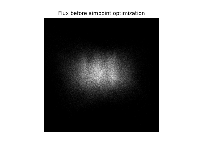
The Effect of Motor Position Optimization

To better understand why motor position optimization is important let’s consider a small example. Receivers are designed and constructed with a known optimal distribution in mind. This distribution might be a homogenous distribution or something similar. The aim is to realize this optimal distribution with all heliostats in the field. Here, we aim to achieve a uniform distribution. However, the flux distribution before motor position optimization is clearly uneven:

During motor position optimization, the heliostats are adjusted to aim at slightly different points on the receiver. This improves the uniformity of the flux distribution on the receiver:

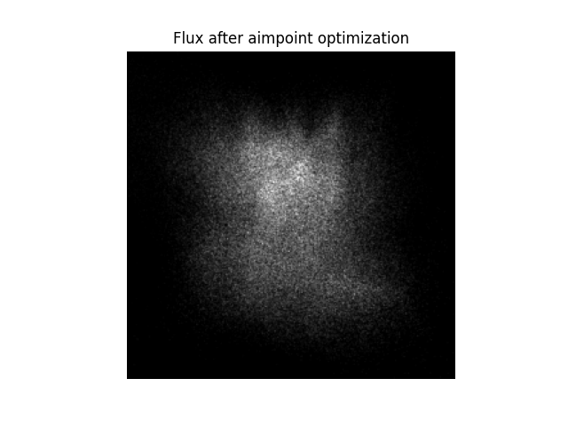
Despite only a few heliostats being present in this scenario, the flux distribution is visibly more uniform after the optimization. Note that due to the small number of heliostats, it is impossible to actually achieve the desired uniform flux distribution – but we clearly see that the flux after the optimization is more broadly distributed than before.