`ARTIST` Tutorial: Kinematics Reconstruction

Note

You can find the corresponding Python script for this tutorial here: https://github.com/ARTIST-Association/ARTIST/blob/main/tutorials/04_kinematics_reconstruction_tutorial.py

This tutorial explains how kinematics reconstruction is performed in ARTIST. In particular, it covers:

why kinematics reconstruction is necessary,
how to load the required calibration data, and
how to configure and run the KinematicsReconstructor.

Before starting this tutorial, make sure you already know how to load a scenario, run ARTIST in a distributed environment for ray tracing, and understand the structure of a scenario. If you are not using your own scenario, we recommend using one of the following scenarios provided in the scenarios/ folder:

test_scenario_paint_multiple_heliostat_groups_ideal.h5
test_scenario_paint_multiple_heliostat_groups_deflectometry.h5

Kinematics Reconstruction Basics

In real heliostats, the components of the kinematic system exhibit small mechanical imperfections. As a result, when an actuator is instructed to orient a heliostat along a specific angle, the heliostat might not point exactly at the intended aim point, while the in-silico heliostats in our digital twin follow the commanded orientation perfectly. To produce accurate predictions in ARTIST, the real-world mechanical deviations must be taken into account. This is what happens during kinematics reconstruction: We learn the offset and deviation parameters of the heliostat’s kinematic system, allowing the simulated heliostat to reproduce the behavior observed in reality more accurately.

Loading the Calibration Data

Reconstructing the kinematics in ARTIST requires calibration data. In this tutorial we use calibration data from the PAINT database. Multiple heliostats can be reconstructed simultaneously, and each heliostat can use several calibration measurements.

Each calibration measurement consists of calibration properties (stored in a .json file) and a measured flux image (stored as .png). As in the surface reconstruction tutorial, this information is provided through a heliostat_data_mapping list of tuples. Each tuple contains the heliostat’s name together with the paths to its calibration data files:

# Please use the following style: list[tuple[str, list[pathlib.Path], list[pathlib.Path]]]
heliostat_data_mapping: list[tuple[str, list[pathlib.Path], list[pathlib.Path]]] = [
(
    "heliostat_name_1",
    [
        pathlib.Path(
            "please/insert/the/path/to/the/paint/data/here/calibration-properties.json"
        ),
        # ....
    ],
    [
        pathlib.Path("please/insert/the/path/to/the/paint/data/here/flux.png"),
        # ....
    ],
),
(
    "heliostat_name_2",
    [
        pathlib.Path(
            "please/insert/the/path/to/the/paint/data/here/calibration-properties.json"
        ),
        # ....
    ],
    [
        pathlib.Path("please/insert/the/path/to/the/paint/data/here/flux.png"),
        # ....
    ],
),
# ...
]

This mapping is stored in a data dictionary that will later be used during optimization:

# Create dict for the data parser and the heliostat_data_mapping.
data: dict[
    str,
    CalibrationDataParser | list[tuple[str, list[pathlib.Path], list[pathlib.Path]]],
] = {
    constants.data_parser: data_parser,
    constants.heliostat_data_mapping: heliostat_data_mapping,
}

If you are not using your own data, you can use the sample data provided in the data/ directory, for example, for heliostats AA31, AA39, and AC43.

Next, load the scenario and set up the distributed environment as in previous tutorials.

Configuring Optimizer and Scheduler

As in the surface reconstruction tutorial, the kinematics reconstructor uses the torch.optim.Adam optimizer. Again, we must define the optimizer parameters and configure a learning rate scheduler. In the kinematics reconstruction, the optimizable parameters are learned using three different learning rates. Since each parameter has its own scale and magnitude, they must be treated separately:

# Configure the optimization.
optimizer_dict = {
    constants.initial_learning_rate_rotation_deviation: 1e-4,
    constants.initial_learning_rate_initial_angles: 1e-3,
    constants.initial_learning_rate_initial_stroke_length: 1e-2,
    constants.tolerance: 0.0000,
    constants.max_epoch: 200,
    constants.batch_size: 50,
    constants.log_step: 1,
    constants.early_stopping_delta: 1e-8,
    constants.early_stopping_patience: 1000,
    constants.early_stopping_window: 2000,
}
# Configure the learning rate scheduler.
scheduler_dict = {
    constants.scheduler_type: constants.reduce_on_plateau,
    constants.gamma: 0.9,
    constants.lr_min: 1e-6,
    constants.lr_max: 1e-3,
    constants.step_size_up: 500,
    constants.reduce_factor: 0.0001,
    constants.patience: 50,
    constants.threshold: 1e-3,
    constants.cooldown: 10,
}
# Combine configurations.
optimization_configuration = {
    constants.optimization: optimizer_dict,
    constants.scheduler: scheduler_dict,
}

With these parameters defined, we are ready to set up the kinematics reconstructor.

Setting up the `KinematicsReconstructor`

To perform kinematics reconstruction, we create a KinematicsReconstructor object. Currently, ARTIST provides one reconstruction method based on differentiable ray tracing. This method uses

the centers of the measured flux density distributions and
the incident ray directions during the measurements.

The reconstructor can be initialized as follows:

kinematics_reconstructor = KinematicsReconstructor(
    ddp_setup=ddp_setup,
    scenario=scenario,
    data=data,
    optimization_configuration=optimization_configuration,
    reconstruction_method=constants.kinematics_reconstruction_raytracing,
)

Performing Reconstruction

The setup is now complete and the kinematics reconstruction can begin. Since the process is formulated as an optimization problem, we must first define the loss function. In this tutorial, we use the FocalSpotLoss, which compares the predicted and measured focal spot locations:

loss_definition = FocalSpotLoss(scenario=scenario)

Now we can perform the reconstruction with the reconstruct_kinematics() method:

final_loss_per_heliostat = kinematics_reconstructor.reconstruct_kinematics(
    loss_definition=loss_definition, device=device
)

The method returns the loss per heliostat as a flattened tensor, which can be used for logging or further analysis.

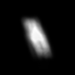
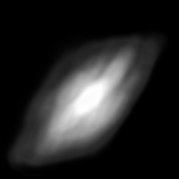
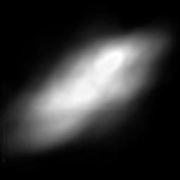
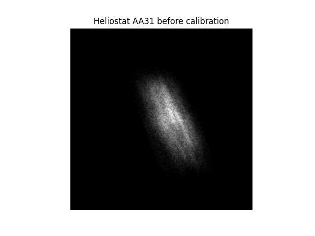
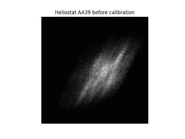
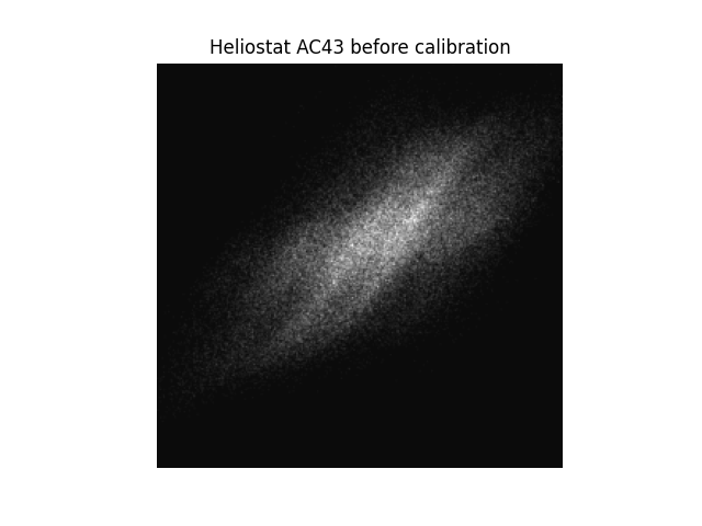
What Happens During the Reconstruction?

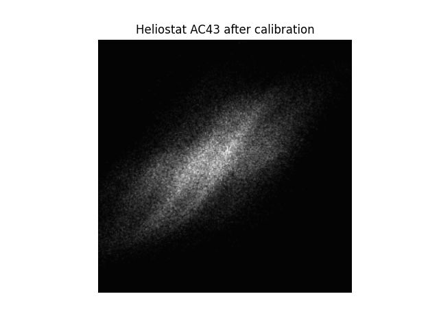
To illustrate the effect of kinematics reconstruction, consider a scenario with three heliostats: AA31, AA39, and AC43.

Target fluxes (row 1), simulated fluxes before kinematics reconstruction (row 2), and simulated fluxes after kinematics reconstruction (row 3).

When we perform ray tracing without prior kinematics reconstruction, the simulated flux distributions differ from the measured ones (compare row 1 and 2):

The simulated flux images have lower resolution than the measured images (which is expected).
The overall shapes of the flux distributions are similar.
The focal spots are not perfectly aligned.

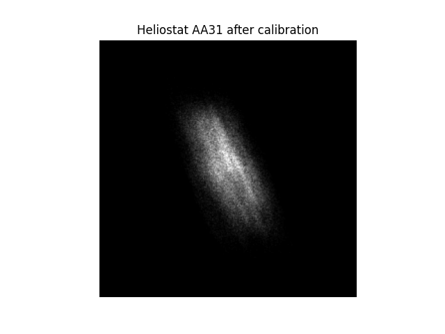
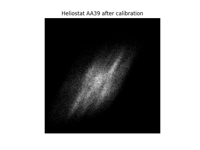
During kinematics reconstruction, ARTIST learns the real-world mechanical imperfections of the heliostat system. After reconstruction, the simulated focal spots shift slightly and align more closely with the measured flux distributions (compare rows 1 and 3). Although the adjustments are small, they significantly improve the agreement between simulation and measurement. At this point, the heliostat kinematics can be considered successfully reconstructed.

Note

The images generated in this tutorial are for illustrative purposes, often with reduced resolution and without hyperparameter optimization. Therefore, they should not be taken as a measure of the quality of ARTIST. Please see our publications for further information.

ARTIST Tutorial: Kinematics Reconstruction