`ARTIST` Tutorial: Motor Position Optimization

Note

You can find the corresponding Python script for this tutorial here: https://github.com/ARTIST-Association/ARTIST/blob/main/tutorials/05_motor_positions_optimizer_tutorial.py

This tutorial introduces the process of optimizing heliostat motor positions using the ARTIST software. This is crucial for precise alignment and maximizing the efficiency of the power plant.

The tutorial will walk you through the key concepts needed to perform this optimization, including:

How to define the ground truth and the loss function.
How to configure the optimization parameters.
How to perform the motor positions optimization.

Before starting this scenario make sure you already know how to load a scenario, run ARTIST in a distributed environment, and understand the structure of a scenario. If you are not using your own scenario, we recommend using one of the “test_scenario_paint_multiple_heliostat_groups_deflectometry.h5” or “test_scenario_paint_multiple_heliostat_groups_ideal.h5” scenarios provided in the “scenarios” folder.

Before getting started, you need to load the scenario and set up the distributed environment, as in previous tutorials.

Motor position optimization aims to optimize the motor positions of multiple heliostats to achieve a desired flux density on the solar tower. In this case, we focus on achieving a trapezoid distribution on the receiver, which is equivalent to all areas of the receiver receiving the same amount of sunlight. This would lead to and optimal flux distribution and improve operation of the power plant. Therefore, we have to define the ground truth with a trapezoid distribution and also set the loss function as the KLDivergenceLoss:

e_trapezoid = utils.trapezoid_distribution(
    total_width=256, slope_width=30, plateau_width=180, device=device
)
u_trapezoid = utils.trapezoid_distribution(
    total_width=256, slope_width=30, plateau_width=180, device=device
)
ground_truth = u_trapezoid.unsqueeze(index_mapping.unbatched_bitmap_u) * e_trapezoid.unsqueeze(index_mapping.unbatched_bitmap_e)
loss_definition = KLDivergenceLoss()

The KLDivergenceLoss measures how one probability distribution is different from a second, reference distribution. In this case the reference distribution is the trapezoid distribution, which we compare to the collective distribution generated by all heliostats in the scenario.

Before we can perform the optimization, we also need to define the learning rate scheduler and the optimizer configuration. Internally, the torch.optim.Adam optimizer is used, but the optimal parameters may differ depending on the data or specific use case. In this tutorial we define the following scheduler and optimization configuration:

scheduler = (
    config_dictionary.exponential
)
scheduler_parameters = {
    config_dictionary.gamma: 0.9,
    config_dictionary.min: 1e-6,
    config_dictionary.max: 1e-3,
    config_dictionary.step_size_up: 500,
    config_dictionary.reduce_factor: 0.3,
    config_dictionary.patience: 10,
    config_dictionary.threshold: 1e-3,
    config_dictionary.cooldown: 10,
}

# Set optimizer parameters.
optimization_configuration = {
    config_dictionary.initial_learning_rate: 1e-3,
    config_dictionary.tolerance: 0.0005,
    config_dictionary.max_epoch: 50,
    config_dictionary.log_step: 10,
    config_dictionary.early_stopping_delta: 1e-4,
    config_dictionary.early_stopping_patience: 10,
    config_dictionary.scheduler: scheduler,
    config_dictionary.scheduler_parameters: scheduler_parameters,
}

Now we are finally done, the final step is to create a MotorPositionsOptimizer object and to run the optimize() method to perform the actual optimization.

# Create the motor positions optimizer.
motor_positions_optimizer = MotorPositionsOptimizer(
    ddp_setup=ddp_setup,
    scenario=scenario,
    optimization_configuration=optimization_configuration,
    incident_ray_direction=torch.tensor([0.0, 1.0, 0.0, 0.0], device=device),
    target_area_index=1,
    ground_truth=ground_truth,
    bitmap_resolution=torch.tensor([256, 256], device=device),
    device=device,
)

# Optimize the motor positions.
_ = motor_positions_optimizer.optimize(
    loss_definition=loss_definition, device=device
)

The optimize() method returns the final loss of the optimization process, which can be useful for logging or analysis. That is all there is to motor position optimization in ARTIST.

The Effect of Motor Position Optimization

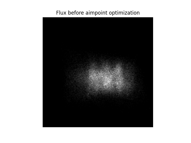
To better understand why motor position optimization is important lets consider a small example. Each receiver is is designed and constructed with a known optimal distribution in mind. This distribution might be a homogenous distribution or something similar. The aim is to realize this optimal distribution with all available heliostats. In the current tutorial, we aim to achieve a uniform distribution, but as we see in the following image, this is clearly not the case:

However, after performing the motor position optimization the various heliostats in the scenario can be pointed to slightly different targets to better approximate the desired distribution. We see this, in the image below:

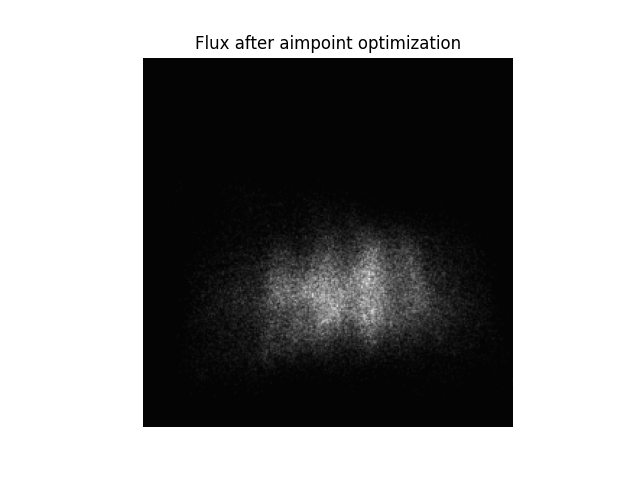
Since only a small number of heliostats are present in this scenario, it is impossible to actually achieve the desired uniform flux distribution - but we clearly see (despite only a few heliostats being present) that the flux is now more broadly distributed than before.

Note

The images generated in this tutorial are for illustrative purposes, often with reduced resolution and without hyperparameter optimization. Therefore, they should not be taken as a measure of the quality of ARTIST. Please see our publications for further information.

ARTIST Tutorial: Motor Position Optimization

The Effect of Motor Position Optimization

`ARTIST` Tutorial: Motor Position Optimization