`ARTIST` Tutorial: Kinematic Reconstruction

Note

You can find the corresponding Python script for this tutorial here: https://github.com/ARTIST-Association/ARTIST/blob/main/tutorials/04_kinematic_reconstruction_tutorial.py

This tutorial explains how kinematic reconstruction is performed in ARTIST, specifically we will look at:

Why do we need to reconstruction the kinematic?
How to load calibration data.
How to set up the KinematicReconstructor responsible for the kinematic reconstruction.

Before starting this scenario make sure you already know how to load a scenario, run ARTIST in a distributed environment for raytracing, and understand the structure of a scenario. If you are not using your own scenario, we recommend using one of the “test_scenario_paint_multiple_heliostat_groups_ideal.h5” or “test_scenario_paint_multiple_heliostat_groups_deflectometry.h5” scenarios provided in the “scenarios” folder.

Kinematic Reconstruction Basics

In the real world most components of the kinematic have mechanical errors. This means if we tell an actuator to orient a heliostat along a specific angle, the heliostat might not end up pointing exactly at the specified aim point. In ARTIST we create a digital twin of a solar tower power plant. In the computer simulation, the heliostat will, per default, point exactly where we tell it to. To keep the predictions made with ARTIST as accurate as possible we need to consider the mechanical errors and offsets of the real-world kinematic. In the kinematic reconstruction process the kinematic module learns all offset or deviation parameters of the real-world kinematic, to mimic its behavior.

Loading the Calibration Data

Reconstructing the kinematic in ARTIST requires calibration data. In this tutorial we consider calibration data from the PAINT database: https://paint-database.org/. Multiple heliostats can be reconstructed simultaneously and each heliostat can be reconstructed with multiple calibration data points at once.

Calibration data consists of calibration properties and a flux image. We load this data with a mapping, analog to the approach shown in the tutorial on surface reconstruction. Specifically, we create a heliostat_data_mapping list of tuples, where each tuple contains the heliostat’s name and the paths to its calibration data, which include both a .json file with calibration properties and a .png flux image:

# Please use the following style: list[tuple[str, list[pathlib.Path], list[pathlib.Path]]]
heliostat_data_mapping: list[tuple[str, list[pathlib.Path], list[pathlib.Path]]] = [
(
    "heliostat_name_1",
    [
        pathlib.Path(
            "please/insert/the/path/to/the/paint/data/here/calibration-properties.json"
        ),
        # ....
    ],
    [
        pathlib.Path("please/insert/the/path/to/the/paint/data/here/flux.png"),
        # ....
    ],
),
(
    "heliostat_name_2",
    [
        pathlib.Path(
            "please/insert/the/path/to/the/paint/data/here/calibration-properties.json"
        ),
        # ....
    ],
    [
        pathlib.Path("please/insert/the/path/to/the/paint/data/here/flux.png"),
        # ....
    ],
),
# ...
]

This data is then saved into a data dictionary which will be later used in the optimization:

# Create dict for the data parser and the heliostat_data_mapping.
data: dict[
    str,
    CalibrationDataParser | list[tuple[str, list[pathlib.Path], list[pathlib.Path]]],
] = {
    config_dictionary.data_parser: data_parser,
    config_dictionary.heliostat_data_mapping: heliostat_data_mapping,
}

If you are not using your own data, you can use the sample data provided in the “data”, for example for the heliostats AA31, AA39, and AC43.

Next, you can load the scenario and set up the distributed environment as in previous tutorials.

Configuring Scheduler and Optimizer

As in the surface reconstruction tutorial, the kinematic reconstructor also uses the torch.optim.Adam optimizer. Therefore we again need to define the parameters used for the learning rate scheduler and the optimization configuration:

scheduler = (
    config_dictionary.exponential
)  # exponential, cyclic or reduce_on_plateau
scheduler_parameters = {
    config_dictionary.gamma: 0.9,
    config_dictionary.min: 1e-6,
    config_dictionary.max: 1e-3,
    config_dictionary.step_size_up: 500,
    config_dictionary.reduce_factor: 0.3,
    config_dictionary.patience: 10,
    config_dictionary.threshold: 1e-3,
    config_dictionary.cooldown: 10,
}

# Set optimization parameters.
optimization_configuration = {
    config_dictionary.initial_learning_rate: 0.0005,
    config_dictionary.tolerance: 0.0005,
    config_dictionary.max_epoch: 1000,
    config_dictionary.log_step: 100,
    config_dictionary.early_stopping_delta: 1e-4,
    config_dictionary.early_stopping_patience: 10,
    config_dictionary.scheduler: scheduler,
    config_dictionary.scheduler_parameters: scheduler_parameters,
}

Now we are ready to set up the kinematic reconstructor.

Setting up the `KinematicReconstructor`

Before we can create a KinematicReconstructor object we need to decide which method we want to use to perform reconstruction. Currently there is only one method to reconstruct the kinematic. In this tutorial we optimize using flux density distributions and the differentiable ray tracer.

The centers of the measured flux density distributions,
The incident ray directions during the measurements,

We can create a KinematicReconstructor object responsible for the kinematic reconstruction with:

kinematic_reconstructor = KinematicReconstructor(
    ddp_setup=ddp_setup,
    scenario=scenario,
    data=data,
    optimization_configuration=optimization_configuration,
    reconstruction_method=config_dictionary.kinematic_reconstruction_raytracing,
)

Performing Reconstruction

The set up is now complete and the kinematic reconstruction can begin. The kinematic reconstruction is an optimization process. Before starting the reconstruction we need to define the loss, in this tutorial we use the FocalSpotLoss since we are working with raytracing:

loss_definition = FocalSpotLoss(scenario=scenario)

Now we can simply perform the reconstruction with the reconstruct_kinematic() method:

final_loss_per_heliostat = kinematic_reconstructor.reconstruct_kinematic(
    loss_definition=loss_definition, device=device
)

The reconstruct_kinematic() method returns the loss per heliostat as a flattened tensor, which may be useful for logging or analysis.

What Happens During the Reconstruction?

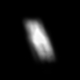
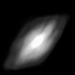
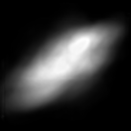
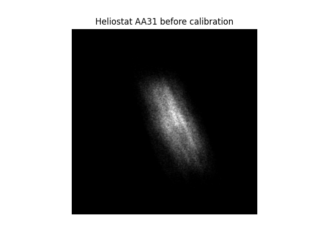
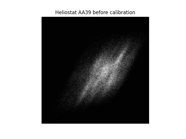
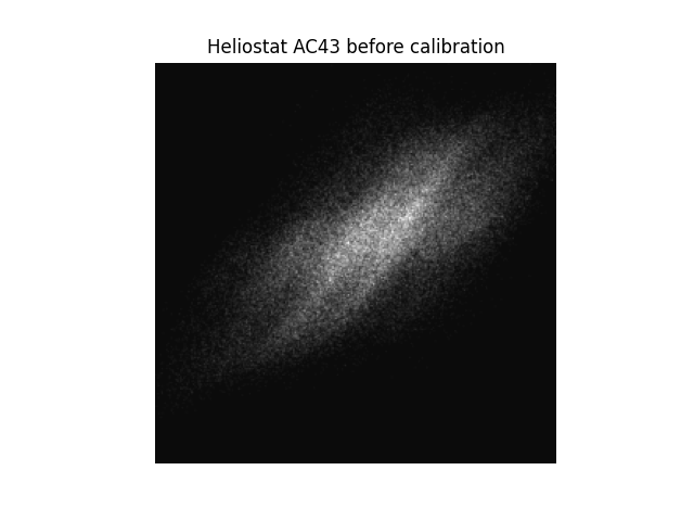
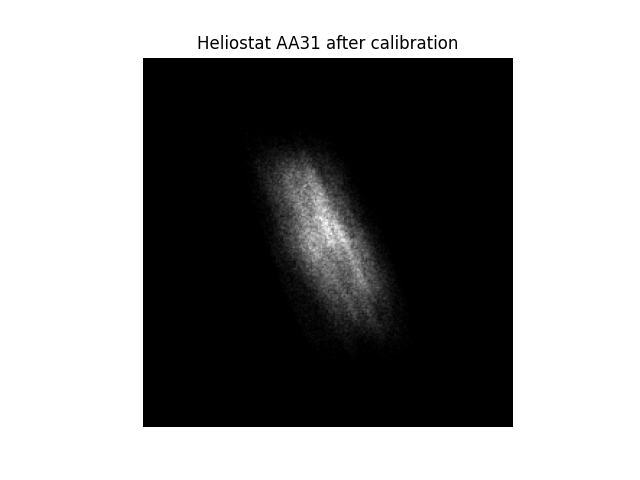
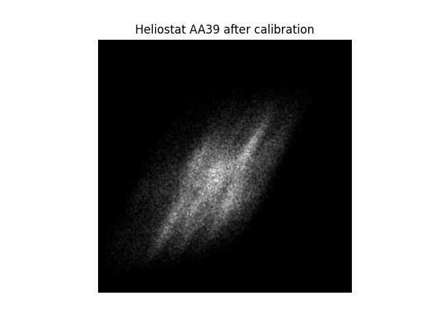
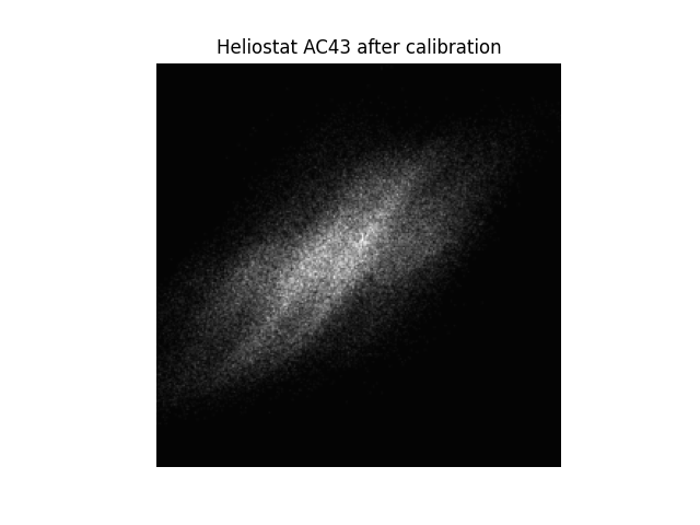
To understand calibration, lets look at a small example based on this tutorial. We were to consider a scenario with three heliostats: AA31, AA39, and AC43.

Target fluxes (row 1), heliostat fluxes before reconstruction (row 2), heliostat fluxes after reconstruction (row 3)

When we perform raytracing without prior kinematic reconstruction and compare the generated fluxes from ARTIST with the fluxes measured on the solar tower during a calibration, as in the first two rows of the images above, we notice, the following:

The resolution of the generated flux images is much lower than in the measured flux images - this is okay.
The shapes of the generated fluxes and the measured fluxes match.
The generated and measured fluxes do not align perfectly.

After the kinematic reconstruction, where the digital twin ARTIST learns the real world imperfections, the generated fluxes in ARTIST have now moved. Whilst the changes are small, it is noticeable that the focal spots are now better aligned with the measured fluxes, compare rows 1 and 3 in the images above. Therefore, we can now consider our heliostat kinematics to be reconstructed - and that is all there is to kinematic reconstruction in ARTIST!

Note

The images generated in this tutorial are for illustrative purposes, often with reduced resolution and without hyperparameter optimization. Therefore, they should not be taken as a measure of the quality of ARTIST. Please see our publications for further information.

ARTIST Tutorial: Kinematic Reconstruction