NURBS in ARTIST
ARTIST uses Non-Uniform Rational B-Splines (NURBS) to model the surface of heliostats for multiple reasons:
NURBS can represent the continuous, complex, and imperfect heliostat surfaces.
NURBS can be differentiable, this enables their parameters to be learned and optimized using AI algorithms.
NURBS representing heliostat surfaces can be constructed with less parameters than constructing heliostat surfaces from point clouds or deflectometry data.
NURBS are precise and performant.
Here we first consider some NURBS Theory before investigating NURBS in ARTIST.
NURBS Theory
In this section, we consider the NURBS theory.
Simplifications
For the sake of simplicity, we only considers NURBS curves and not surfaces.
The behavior of NURBS curves in two dimensions can easily be transferred to NURBS surfaces in three dimensions.
Two NURBS curves can span a NURBS surface.
NURBS are generally parametrized by functions of the form \(Q(t)=\{X(t), Y(t)\}\), where \(t\) can be considered as a variable representing time. For a curve specifically, we can imagine this curve is traced out by a particle moving through space. In this case, \(Q(t)\) gives the \(\{x, y\}\) coordinates of the particle at time \(t\).
Key Components and Characteristics of NURBS
NURBS are made up out of the following components:
Control points,
Basis functions,
Knots,
Weights, and
Degrees
Different manifestations of these components result in different properties of the NURBS, for example, non-uniformity or rationality.
To better understand this, we will consider each of these components and characteristics in more detail.
Degree
The degree is always a positive integer and closely related to the order, specifically:
For example, a third-order curve is represented by quadratic polynomial which results in a quadratic curve. Note that:
It is possible to increase the degree of the NURBS curve without changing its form.
It is not possible to reduce the degree without changing its form.
Control Points
The shape of the NURBS is directly determined by the control points. The most important aspects to remember about control points are:
A higher number of control points, usually allows for a more accurate approximation of a given curve.
The control points are represented as a list of points, importantly the length of this list must be at least \(\text{degree}+1\).
The shape formed by connecting the control points with straight lines is the control polygon.
In the figure below, we see how the control points influence the shape of the NURBS curve.
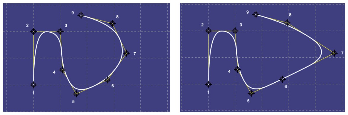
More specifically:
The only parameter that changes between the two curves is the location of control point \(7\).
The change in the curve is limited to the local neighborhood of that control point.
This example demonstrates one key aspect of NURBS: each control point only influences the part of the curve nearest to it and has little or no effect on parts of the curve that are farther away. Considering the example of a particle moving through time from before, we can say that at any time \(t\) the particle´s position is a weighted average of all control points but the points closer to the particle are weighted more than those farther away.
We can express this idea mathematically via
where \(k = \text{order}\) with \(\text{order} = \text{degree} + 1\), \(n = \text{number of control points}\), \(B\) are the control points, and \(N\) represents the basis functions.
Basis Functions
Basis functions are assigned to control points with each control point having a corresponding basis function. Importantly, \(N_{i,k}(t)\) are the basis functions and they determine how strongly the control point \(B_i\) influences the NURBS curve at time \(t\).
To better understand basis functions, let us consider the following image:
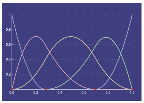
Here we see exemplary basis functions for a NURBS curve with 5 control points. Each control point has one basis function. The red basis function is assigned to control point 2, considering the interval \(t = 0\) to \(t = 0.7\). This is the time interval during which control point 2 controls the shape of the NURBS curve. For \(t = 0.8\), only the basis functions of control point 3, 4 and 5 are activated thus only control points 3, 4, and 5 control the shape of the NURBS curve at that time. Since the green basis function that is assigned to control point 4 peaks at \(t = 0.8\), this control point has the most influence on the NURBS curve at that point in time. Some further important observations include:
At any time \(t\), the values of all basis functions add up to exactly 1.
At any time \(t\), no more than \(k\) basis functions affect the curve (\(k = \text{order} = \text{degree} + 1\)). The example above is of order 3.
A curve of order \(k\) is only defined for periods where \(k\) of the basis functions are non-zero.
In the example above, all control points affect equally sized regions of the curve and also affect the curve with the same strength, thus they are uniform (and have uniform knot vectors).
If this is not desired, then non-uniform NURBS with non-uniform knots must be considered.
In ARTIST, we only apply uniform NURBS. However, for completeness, we should also understand
how to create non-uniform NURBS.
Knots
Knots are a series of points that partition the overall time it takes the particle to move along the curve into intervals. Knots are represented as an ordered list of numbers where
By varying the relative lengths of the intervals, the amount of time each control point affects the particle is varied – also known as the knot spans.
To understand this in more detail, let’s look at some examples. First, a uniform knot vector implies that all knots are equidistant and as a result all basis functions cover equal intervals of time. This is illustrated below:
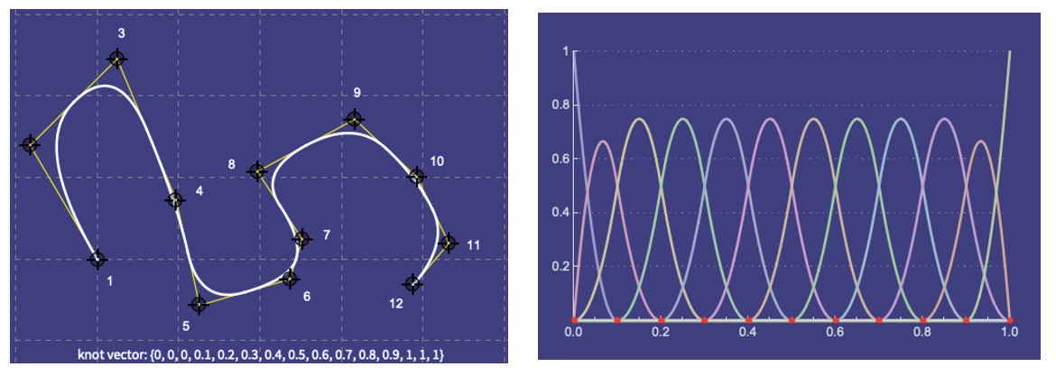
On the other hand, a non-uniform knot vector contains knot spans of different sizes which means that the basis functions cover different intervals of time as shown below:

It is important to note that not all basis functions are the same. Some are taller and some are wider than others. This is because the knot spans vary. For smaller knot spans, the basis functions become taller and narrower. For the corresponding control points, the curve is pulled more strongly to those control points.
Using our knowledge on knots, we can now formulate the following mathematical definition of the basis functions:
where \(x_i\) is the i-th knot in the knot vector.
Knot Span
We already discussed the knot span, however, there are a few important terms we need to define:
If we have a knot span of zero length, i.e., two consecutive knots have the same value, then this is a knot with multiplicity. Importantly, a knot has full multiplicity if \(\text{multiplicity} = \text{degree}\). Furthermore, a simple knot is a knot with a multiplicity of 1.
If the first and last knot have full multiplicity, the NURBS curve begins and ends in a control point. Full multiplicity in the first and last knot does not affect the uniformity property.
Uniformity describes knot vectors that start and end with full multiplicity knots, and contain simple knots with knot spans of the same length inbetween. For example, the knot vector \([0,0,0,1,2,3,4,4,4]\) describes uniformity for a degree of 3.
Control Weights
The last aspect of NURBS we want to consider are the control weights. The control weights are responsible for the rational property of NURBS:
If all control weights are always 1, the NURBS are non-rational which is a special subset of rational NURBS.
If all control weights have a weight of 1, this implies that each control point has an equal influence on the shape of the curve.
Increasing the weight of one control point gives it more influence and “pulls” the curve towards that control point.
Rational curves imply that some or all control weights differ from 1.
Note that in ARTIST all control weights are always 1.
The parametric UV space of 3D NURBS surfaces
Contrary to the rest of ARTIST, the NURBS are defined using variable names ending in \(u\) and \(v\) instead of the
cartesian coordinate naming east, north and up. This is due to the mathematical concept behind the NURBS. NURBS are always defined
in a parametric space, usually called the UV space, where the parameters \(u\) and \(v\) typically range from 0 to 1. Within
this space, the surface is mathematically described through the concepts explained above (basis functions, …). The physical surface
itself does not exist in the 3D cartesian space until it is sampled. During the sampling the east, north, up (or \(x\), \(y\), \(z\))
coordinates are first mapped back into the UV domain so that the parametric basis functions can be evaluated, producing the actual
cartesian surface coordinates. The UV space enables the NURBS to represent smooth, continuous surfaces in a flexible way.
NURBS in ARTIST
Now that we know the basics of NURBS, let us look briefly at how ARTIST makes use of NURBS. Importantly:
The NURBS in
ARTISTare differentiable.They are primarily used to model the heliostat surfaces, however they can also be used to model other surfaces, such as the receiver.
The NURBS in
ARTISTare uniform and non-rational. The name NURBS can therefore be misleading; however, the uniform and non-rational implementation is a subset of NURBS.
Code
The NURBS code in ARTIST is contained in nurbs.py which can be found under artist/util. The nurbs.py module
implements the NURBSSurface class and inherits from torch.nn.Module, allowing for gradient-based calculations.
Usage
Using NURBS in ARTIST is simple:
A NURBS surface can be initialized by only providing the desired
degreesin theuandvdirection, and the associatedcontrol points. For a NURBS surface, two degrees are necessary as two NURBS curves span the surface. Internally, the uniform knot vectors are calculated from the input.The user can then simply call
calculate_surface_points_and_normals()on theNURBSSurfaceand the surface points and surface normals are calculated and returned.
For this calculation of the surface points and surface normals, three internal steps are executed:
find_span()is called for both directions to determine which evaluation point corresponds to which knot in the knot vector.Next, the basis functions and their derivatives are calculated, again for both directions using
basis_function_and_derivatives().Lastly, the surface points and normals are calculated from the basis functions, their derivatives, and the control points.